Aim: To learn the process of bacterial conjugation through the transfer of genes, coding for antibiotic resistance.
Principle: Transfer of genetic material from one bacterial strain (donor) to another strain (recipient) is a common event that occurs in nature with the objective of mixing the gene pool, in otherwise asexually reproducing organisms. DNA transfer among bacteria is mediated in three ways viz., transfection, transduction and conjugation. Conjugation is the most widespread process of transferring genetic material from one bacterial cell to another. It is a process in which unidirectional transfer of DNA is mediated by conjugal plasmids or conjugal transposons requiring cell-to-cell contact. It was discovered by
Lederberg and Tatum in 1946.
Conjugation is best understood by considering properties of the 'F'factor, which is a small circular plasmid DNA that can replicate autonomously in the cell or can integrate into the host chromosome and thus transfer host chromosomal markers. When individual cells with an integrated 'F' are isolated and allowed to form pure colonies, the resulting strain can transfer chromosomal markers at very high frequency and are termed Hfr strains.
Materials Provided:
The list below provides information about the materials supplied in the kit. The products should be stored as suggested. Use the kit within 6 months of arrival.
Materials Required:
Equipment: Incubator, Shaker (37°C), Spectrophotometer.
Glassware: Conical-Flasks, Petri plates, Pipettes, Spreader, Test tubes.
Reagent: Distilled water.
Other Requirements: Cuvette (of 1 cm path length)
Micropipette, Tips.
Note:
Read the entire procedure before-starting the experiment.
All microbiological operations should be done strictly under aseptic conditions.
Revive the strains as soon as the lyophilized vial is opened.
Carry out the experiments within 2 weeks of reviving the strains.
For preparation of media and antibiotic, refer appendix. Bacterial Conjugation
Distinguishing characteristics of conjugation:
ONA transfer requires cell-cell contact.
DNA transfer occurs via a conjugal pore – resistant to DNase.
DNA transfer occurs in one direction - from donor to recipient and not vice versa.
DNA transfer does not require protein synthesis in donor cell.
DNA transfer requires energy in donor cell – primarily ATP.
Appendix:
Preparation of LB Broth/Agar (1 litre): Dissolve 25 g of media in 800 ml of distilled water. Adjust the pH to 7.0 with 5N NaOH (if necessary) and make up the volume to 1000 ml. Sterilize by autoclaving.
For LB agar, add 1.5% agar and autoclave.
Preparation of antibiotic:
Tetracycline: Dissolve 45 mg of tetracycline supplied in 1.5 ml of 70% ethanol, vortex if necessary. This gives a stock concentration of 30 mg/ml. Cover the vial with aluminium foil and store at 4°C. Use the antibiotic solution within 2 weeks. Add this antibiotic solution to LB media at a concentration of 30 mg/ml.
Streptomycin: Dissolve 150 mg of streptomycin supplied in 1.5 ml of sterile water, vortex if necessary. This gives a stock concentration of 100 mg/ml. Cover the vial with
aluminium foil and store at 4°C. Use the antibiotic solution within 2 weeks. Add this antibiotic solution to LB media at a concentration of 100 mg/ml.
Following aliquots of media are required for single conjugation experiment. (Excludes preparation of media for revival of strain).
• LB Broth 6 ml
• LB Broth + Tetracycline 6 ml + 25 ml
• LB Broth + Streptomycin 6 ml + 25 ml
• LB Agar + Tetracycline 60 ml
• LB Agar + Streptomycin 60 ml
• LB Agar + Tet. + Strep. 60 ml
Note: Prepare 25 ml LB Broth in a 100 ml conical flask.
Procedure:
Day 1: Revival of parental strains.
1. Break open one set of lyophilized vials (donor & recipient E. coli strains). Rehydrate each vial with 0.1 ml of sterile LB broth.
2. Streak the donor strain on LB plate with tetracycline (concentration 30 //g/ml),and the recipient strain on LB with streptomycin (concentration 100 //g/ml). (Streak in duplicates).
3. Incubate the plates at 37°C overnight.
Note: Store the revived plates at 4°C,and use within 2 weeks to carry out 5 experiments
in case of KT45.
Day 2:
4. Pick single colony each from the donor and recipient plate and inoculate into 6 ml LB broth containing the respective antibiotic.
5. Incubate at 37°C in a shaker overnight.
Day 3: Conjugation
6. Inoculate 1 ml of overnight donor culture into 25 ml LB broth (in 250 ml conical flask) with tetracycline at a concentration of 30 //g/ml.
7. Incubate at 37°C in a shaker.
8. Inoculate 3 ml of overnight recipient culture into 25 ml LB broth (in 250 ml conical flask) with streptomycin at a concentration of 100//g/ml.
9. Incubate at 37°C in a shaker.
10. Grow recipient and donor cultures till the O.D. of the donor culture reaches 0.8 - 0.9 at A600.
11. Take 0.2 ml each of donor and recipient cultures in a sterile cotton plugged test tube for conjugation. Label this as conjugated sample.
12. Gently mix and incubate in an incubator at 37°C for 11/2hr-2hrs.
13. Pipette 0.2 ml each of donor and recipient cultures into two different test tubes and Incubate at 37°C for 11/2 hrs.
14. Add 2 ml of sterile LB into each tube after 11/2, hours of incubation.
15. Incubate the tubes at 37°C for another 11/2 hrs.
Note: Do not place the tubes in a shaker during conjugation or subsequent incubation
Period.
16. Spread plate 0.1 ml of each of the samples (donor, recipient, conjugated sample) on antibiotic plates as indicated in the table.
17. Incubate the plates at 37°C overnight.
Observation: Tabulate your observations as follows for each experiment:
Note: Denote positive on observing bacterial growth and negative on seeing no growth.
Interpretation:
From the observations, one can interpret that:
Donor (Tef) and the recipient (Strep') grow only on those antibiotic plates to which they are resistant.
Donor and Recipient being sensitive to Streptomycin and Tetracycline respectively will not grow on those antibiotic plates.
Conjugated sample grow on Tetracycline and Streptomycin LB plate. This is because there is gene transfer of antibiotic resistance from F factor of donor to recipient via the process of conjugation. On the other hand, both the parental strains do not grow on the double antibiotic plate as it contains one or the other antibiotic to which they are sensitive.Bacterial lawn is also seen on plating conjugated sample on the individual antibiotic plates.
Thursday, April 19, 2007
Counter current immunoelectrophoresis
AIM: To check antisera for the presence and specifity of antibodies for a particular antigen by Counter current immunoelectrophoresis.
INTRODUCTION
Counter current immunoelectrophoresis (CCIEP) is a rapid version of Ouchterlony double diffusion (ODD) technique. The technique is used to check antisera for the presence and specificity of antibodies for a particular antigen.
PROCEDURE
Prepare10 ml of 1.5% agarose(0.15g/10ml) in 1X reservoir buffer by adding dry agarose to the buffer and heating slowly to dissolve the agarose completely.
Mark the end of the slide that will be towards positive electrode during the electrophoresis.
Place the slide on a leveled tabletop and quickly pipette 7ml agarose onto 50X75mm slide, spreading while releasing the agarose. Allow solidifying for 15min.
Place the gel plate on the template holder and fix it for CCIEP. Punch 3mm wells with the gel punch at position indicated for CCIEP.
Place the slide in electrophoresis tank and fill the tank with buffer.
Add 10 l of antigen in the four wells towards –ve electrode and 10 l of positive control antiserum and three test antisera in wells towards positive electrode.
Apply 50v and allow the electophoresis to continue for about 45 min.
Observe for precipitin line between the antigen and antisera wells.
Observation:
Here, pattern shows precipitin line between antigen and antisera wells.
INTERPRETATION
Precipitin line indicates the presence of antibody the antigen in the test sera.
The presence of more than one precipitin lines indicate the heterogenicity of the antibody for the antigen in the test sera.
The absence of the precipitin line indicates the absence of any antibody for the antigen in the test sera
Immuno histochemistry
Aim: To perform staining of tissue sections using antibodies (immuno histochemistry)
Principle: Antigen - antibody interactions form the basis of several techniques used in modern day scientific research and in routine clinical diagnosis. One such technique immunohistochemistry is used for the localization of an antigen in a cell or tissue using a specific antibody. The antibody binds specifically to the antigen present in the cell and the antigen-antibody complex is detected using an enzyme - linked secondary antibody. Addition of the substrate for the enzyme forms an insoluble colored precipitate in the tissues and allows localization of antigens.In Immunohistochemistry, sections of fixed, paraffin embedded tissue of interest are taken on glass slides. Fixation preserves the morphology of the cells/tissues as well as keeps the antigen from degrading. Paraffin has to be removed in order to allow the antibody to penetrate the tissue cells and bind to the antigen. This is achieved by using xylene. Antibodies are liquids and will not bind to the antigen unless the dry sections are hydrated. Hence the need to gradually introduce water in the cells of the tissues through grades of alcohol. Phosphate Buffered Saline (PBS) maintains the physiological pH ideal for any antigen-antibody reaction. The blocking step avoids any non-specific binding of the primary antibody. Most tissues express the enzyme Horse Radish Peroxidase endogenously. Hence H2O2. PBST and PBS washes remove excess of unbound antibody (Primary/Secondary) and maintain the PH.
Procedure:
Day 1: Deparafinizing, rehydrating and blocking
Deparaffinize the sections by placing the slide in Coplin jar with xylene for 10 minutes.
Transfer to a second Coplin jar of Xylene and keep the slides for 10 minutes.
Rehydrate the sections by passing the slide through various grades of alcohol viz. Absolute, 90%, 80% and 70% for 10 minutes in each jar.
Dip the sections in 1X PBS.
Place the slide in a moist chamber with sections facing upwards and cover each section with 100 µl of blocking serum. Incubate for 1 hour at room temperature (RT).
Rinse the slide in a jar of PBS.
Return slide to the moist chamber. Block endogenous peroxidase in the tissue sections by covering each of the sections with 100 l of freshly prepared mixture of methanol and 3% H2O2 in the ratio 4:1. (Add 200µl methanol to 50 µl 3% H2O2 in a 1.5 ml vial). Incubate for 30 minutes at RT.
Rinse the slide in a jar of fresh PBS.
Return slide to the moist chamber. To one section add 100µl of primary antibody. To the other section add 100 µl of negative control antibody. Incubate overnight at 4°C. (Cover the box and leave it in the refrigerator). Please note the orientation of the Sections in your observation book.
Day 2: Staining and mounting
Drain the antibody solutions on tissue paper. Place in a coplin iar with PBST. Wash 3 times with fresh PBST for 10 minutes each, followed by 3 washes in a fresh jar of PBS for 10 minutes each. (You may keep the coplin jar on a rocking platform).
Place the slide in the moist chamber. Add 100 pi of djjuted secondary antibody to each section and incubate for 1 hour at RT. (Do not exceed 1 hour incubation. It can increase non-specific reaction).
Transfer the slide to fresh PBST and wash for 10 minutes. Give 3 washes of 10 minutes each, followed by 3 washes with PBS of 10 minute each.
Wipe excess PBS around the sections. Keep the slide on a flat surface. Add 100 µl of substrate to each section and observe for colour development. (Do not exceed 10 minutes. Avoid exposure to direct light).
Stop the reaction by placing the slide in a jar of PBS.
Counter stains the sections by adding 100 µl of Hematoxylin to each section for 30 seconds.
Wash the slide under slow running tap water for 5 minutes by placing them in a coplin jar.
Dehydrate the sections by passing them through increasing grades of alcohol viz., 70% alcohol, 80% alcohol, 90% alcohol and absolute alcohol for 10 minutes in each.
Clear the sections by placing them in a jar of Xylene for 10 minutes.
Transfer to a second jar of Xylene for 10 minutes.
Mount the sections by placing a drop of DPX mountant on them and slowly dropping a coverslip on it (no air bubbles should be present).
Allow drying for half an hour.
Observe the staining under a light microscope.
Observation:
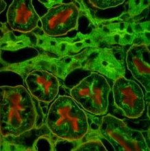
Observe the staining pattern of epithelial cells in both the sections and note the differences. The margins of epithelial cells show brown staining with primary antibody. Negative control antibody does not show this pattern. Nuclei of all cells stain blue with Hematoxylin.
Interpretation:
In the section stained with the primary antibody, the margins of most of the epithelial cells are stained brown indicating the presence of the antigen in the membranes of epithelial cells. This staining pattern is not observed in the section stained with the negative control antibody. The primary antibody specifically localizes the antigen present in the membranes of epithelial cells.
Principle: Antigen - antibody interactions form the basis of several techniques used in modern day scientific research and in routine clinical diagnosis. One such technique immunohistochemistry is used for the localization of an antigen in a cell or tissue using a specific antibody. The antibody binds specifically to the antigen present in the cell and the antigen-antibody complex is detected using an enzyme - linked secondary antibody. Addition of the substrate for the enzyme forms an insoluble colored precipitate in the tissues and allows localization of antigens.In Immunohistochemistry, sections of fixed, paraffin embedded tissue of interest are taken on glass slides. Fixation preserves the morphology of the cells/tissues as well as keeps the antigen from degrading. Paraffin has to be removed in order to allow the antibody to penetrate the tissue cells and bind to the antigen. This is achieved by using xylene. Antibodies are liquids and will not bind to the antigen unless the dry sections are hydrated. Hence the need to gradually introduce water in the cells of the tissues through grades of alcohol. Phosphate Buffered Saline (PBS) maintains the physiological pH ideal for any antigen-antibody reaction. The blocking step avoids any non-specific binding of the primary antibody. Most tissues express the enzyme Horse Radish Peroxidase endogenously. Hence H2O2. PBST and PBS washes remove excess of unbound antibody (Primary/Secondary) and maintain the PH.
Procedure:
Day 1: Deparafinizing, rehydrating and blocking
Deparaffinize the sections by placing the slide in Coplin jar with xylene for 10 minutes.
Transfer to a second Coplin jar of Xylene and keep the slides for 10 minutes.
Rehydrate the sections by passing the slide through various grades of alcohol viz. Absolute, 90%, 80% and 70% for 10 minutes in each jar.
Dip the sections in 1X PBS.
Place the slide in a moist chamber with sections facing upwards and cover each section with 100 µl of blocking serum. Incubate for 1 hour at room temperature (RT).
Rinse the slide in a jar of PBS.
Return slide to the moist chamber. Block endogenous peroxidase in the tissue sections by covering each of the sections with 100 l of freshly prepared mixture of methanol and 3% H2O2 in the ratio 4:1. (Add 200µl methanol to 50 µl 3% H2O2 in a 1.5 ml vial). Incubate for 30 minutes at RT.
Rinse the slide in a jar of fresh PBS.
Return slide to the moist chamber. To one section add 100µl of primary antibody. To the other section add 100 µl of negative control antibody. Incubate overnight at 4°C. (Cover the box and leave it in the refrigerator). Please note the orientation of the Sections in your observation book.
Day 2: Staining and mounting
Drain the antibody solutions on tissue paper. Place in a coplin iar with PBST. Wash 3 times with fresh PBST for 10 minutes each, followed by 3 washes in a fresh jar of PBS for 10 minutes each. (You may keep the coplin jar on a rocking platform).
Place the slide in the moist chamber. Add 100 pi of djjuted secondary antibody to each section and incubate for 1 hour at RT. (Do not exceed 1 hour incubation. It can increase non-specific reaction).
Transfer the slide to fresh PBST and wash for 10 minutes. Give 3 washes of 10 minutes each, followed by 3 washes with PBS of 10 minute each.
Wipe excess PBS around the sections. Keep the slide on a flat surface. Add 100 µl of substrate to each section and observe for colour development. (Do not exceed 10 minutes. Avoid exposure to direct light).
Stop the reaction by placing the slide in a jar of PBS.
Counter stains the sections by adding 100 µl of Hematoxylin to each section for 30 seconds.
Wash the slide under slow running tap water for 5 minutes by placing them in a coplin jar.
Dehydrate the sections by passing them through increasing grades of alcohol viz., 70% alcohol, 80% alcohol, 90% alcohol and absolute alcohol for 10 minutes in each.
Clear the sections by placing them in a jar of Xylene for 10 minutes.
Transfer to a second jar of Xylene for 10 minutes.
Mount the sections by placing a drop of DPX mountant on them and slowly dropping a coverslip on it (no air bubbles should be present).
Allow drying for half an hour.
Observe the staining under a light microscope.
Observation:
Observe the staining pattern of epithelial cells in both the sections and note the differences. The margins of epithelial cells show brown staining with primary antibody. Negative control antibody does not show this pattern. Nuclei of all cells stain blue with Hematoxylin.
Interpretation:
In the section stained with the primary antibody, the margins of most of the epithelial cells are stained brown indicating the presence of the antigen in the membranes of epithelial cells. This staining pattern is not observed in the section stained with the negative control antibody. The primary antibody specifically localizes the antigen present in the membranes of epithelial cells.
Rocket immuno-electrophoresis (RIEP)
Aim: To perform rocket immuno-electrophoresis (RIEP) for the determination of various concentration of antigen in given unknown sample.
Principle: Rocket Immunoelectrophoresis (RIEP) also known, as electro-immuno diffusion is a simple, quick and reproducible method for determining the concentration of antigen (Ag) in an unknown sample. Various concentrations of antigen are loaded side by side in small circular wells along the edge of an agarose gel that contains the specific antibody (Ab). On electrophoresis, the antigen begins to migrate towards the anode and interacts with antibody molecules to form a soluble antigen-antibody complex. However, as the samples electrophorese farther through the gel, more antibody molecules are encountered that interact with the antigen and when the "equivalence point" is reached, the Ag-Ab complex precipitates. This precipitin line is seen in the form of a rocket.
Higher the amount of antigen loaded in the well, farther the antigen will travel through the gel. Hence, with increasing antigen concentration, a series of rockets of increasing heights are seen that is proportional to amount of antigen in the well. Therefore, a direct measurement of the height of rocket will reflect upon the antigen concentration. A standard graph of antigen concentration versus peak height is then constructed and from the peak height of the unknown sample, concentration of antigen is determined.
Material Required: Conical flask, measuring cylinder, alcohol, distilled water, micro pipette, micro tips
Material provided:
Standard antigen: BSA A: 0.0125 mg/ml
B: 0.25 mg/ml
C: 1mg/ml
Antiserum: Goat anti BSA
Procedure:
1. Prepare 10 ml of 1.0% agarose (0.1 g/10 ml) in 1X electrophoresis buffer by heating slowly till agarose dissolves completely. Take care not to scorch or front the solution.
2. Allow the molten agarose to cool to 55°C.
3. Add 1 ml of antiserum to 10 ml of agarose solution. Mix gently, ensure uniform distribution of antiserum.
4. Pour the mix onto a glass plate placed on a horizontal surface and allow it to gel/solidify.
5. Place the glass plate on the template holder provided (in ETS-2) and fixes the RIEP template.
6. Punch 3 mm wells with gel puncher towards one edge of the plate.
7. Place the glass plate in the electrophoresis tank; ensure that the wells are towards the cathode.
8. Fill the tank with 1X electrophoresis buffer till it covers the gel.
9. Connect the power cord to the electrophoretic power supply according to the convention: Red: anode and Black: cathode.
10. Add 10/71 each of the given standard antigen and test antigen to the wells. Loading of wells should be carried out quickly to minimize diffusion from the well.
11. Electrophoreses the samples at 100 volts, till the rockets are visible or the dye front reaches the edge. This generally takes 1 to 11/^ hours. Electrophoresis can be continued for an additional 15 minutes after the dye has run out of the gel. This ensures better visibility of the precipitation peaks.
12. Stop electrophoresis; remove the glass plate from the electrophoresis tank.
13. Observe the precipitation peak or rocket formed against a dark background. If the rockets are still not clear; incubate the plate in a moist chamber at room temperature for 1 hour to overnight.
14. Measure the rocket height from the upper edge of the well to the tip of the rocket. Record your observations as in table 1.
15. Construct a standard graph by plotting the height of the rocket on Y-axis (linear scale) against the concentration of antigen on X-axis (log scale) on a semi-log graph sheet.
16. Determine the concentration of antigen in the test sample by reading the concentration against the rocket height from the standard graph.
Observation:
Result and discussion:
Initially the gel is prepared in given 1xPBS buffer add and adequate amount of anti serum to that and spread it on a plate and allow it to settle than make wells and to each well add the adequate quantity of the standard and test antigen then allow the gel to run through electrophoresis at 100 Volts up to 1 hour. A pattern of rocket is observed. Put the result in the table and plot the graph using the observed result. From the graph calculate the concentration of unknown. From the graph concentration of unknown test sample 1 and2 is found to be 0.81 and 0.75 mg/ml respectively.
Radial immunodiffusion technique for the quantitative analysis of the given antigen
Aim :- Radial immunodiffusion technique for the quantitative analysis of the given antigen.
Principle:Single radial immunodiffusion (RID) is used extensively for the quantitative estimation of antigens. The antigen-antibody precipitation is made more sensitive by the incorporation of antiserum in the agarose. Antigen (Ag) is then allowed to diffuse from wells cut in the gel in which the antiserum is uniformly distributed. Initially, as the antigen diffuses out of the well, its concentration is relatively high and soluble antigen-antibody adducts are formed. However, as Ag diffuses farther from the well, the Ag-Ab complex reacts with more amount of antibody resulting in a lattice that precipitates to form a precipitin ring. (Refer fig. 1).
Thus, by running a range of known antigen concentrations on the gel and by measuring the diameters of their precipitin rings, a calibration graph is plotted. Antigen concentrations of unknown samples, run on the same gel can be found by measuring the diameter of precipitin rings and extrapolating this value on the calibration graph.
Materials Required:
Glassware: Conical flask, Measuring cylinder.
Reagents : Alcohol, Distilled water.
Other Requirements : Micropipette, Tips, Moist chamber (box with wet cotton).
Note:
Read the entire procedure before starting the experiment.
· Dilute required amount of 10X assay buffer to 1X with distilled water.
· Reconstitute the antigen vials (standard and test) with 0.35 ml of 1X assay buffer. Mix well and store at 4°C.Use within 3 months.
· Reconstitute antiserum vial with 2 ml of 1X assay buffer. Mix well and store at 4°C. Use within 3 months.
· Wipe the glass plate with alcohol thoroughly to make it grease free for even spreading of agarose.
· Cut the wells neatly without rugged margins to get a perfect ring of precipitation.
· Add the antiserum to agarose only after it cools to 55°C. Higher temperature will inactivate the antibody.
· Assay buffer: Phosphate buffered saline.
Procedure:
1. Prepare 10 ml of 1.0% agarose (0.1 g/10ml) in 1X assay buffer by heating slowly till agarose dissolves completely. Take care not to scorch or froth the solution.
2. Allow the molten agarose to cool to 55°C.
3. Add 120 ml of antiserum to 6 ml of agarose solution. Mix by gentle swirling for uniform distribution of antibody.
4. Pour agarose solution containing the antiserum onto a grease free glass plate set on a horizontal surface. Leave it undisturbed to form a gel
5. Cut wells using a gel puncher as shown in figure 2, using the template provided.
6. Add 20 ml of the given standard antigens and test antigens to the wells.
7. Keep the gel plate in a moist chamber (box containing wet cotton) and incubate overnight at room temperature.
8. Mark the edges of the circle and measure the diameter of the ring. Note down your observations.
9. Plot a graph of diameter of ring (on Y-axis) versus concentration of antigen (on X- axis) on a semi-log graph sheet.
10. Determine concentration of unknown by reading the concentration against the ring diameter from the graph.
Observation:
Result: Initially, an agarose gel was prepared in 1x buffer and dilutions of antigens and antiserum were prepared as per the kit manuals given and antiserum was mixed with the gel and throughout the gel it is well spread. Against this antisera antigens.
Standard antigen A, B, C, D of the concentration (0.25 ,0.5,1.0,2.0mg/ml) and two test antigen 1 and 2 were allowed to diffuse overnight in humid chamber and the ring pattern as shown in the printout attached. The diameter of these ring were measured and graph of the concentration of the antigen Vs the diameter of the ring is plotted on a semi log graph paper and from this standard plot the concentration of unknown was measured by extrapolating the lines from the graph. from the graph the concentration of the unknown is found to be test sample 1-2 1.23 mg/ml and 1.52 mg/ml respectively.
Competitive ELISA.
Aim: To determine concentration of antigen by antigen capture ELISA or competitive ELISA.
Principle: ELISA or enzyme linked immunosorbent assay is a sensitive laboratory method used to detect the presence of antigens (Ag) or antibodies (Ab) of interest in a wide variety of biological samples. These assays require an immunosorbent i.e., antigen or antibody immobilized on solid surface such as wells of microtitre plates or membranes.
Antigen capture ELISA method is the most useful immunosorbent assay for detecting antigen, since it is 2-5 fold more sensitive than those assays in which antigen is directly bound onto the solid phase. In this assay, constant and limiting amount of antibody is immobilized onto a solid support. A fixed amount of labeled antigen [i.e., antigen coupled with enzyme like Horse radish peroxidase (HRP), alkaline phosphatase (ALP) etc.] is added and allowed to compete with unlabeled antigen (standard or test sample) for the immobilized antibody. The amount of labeled antigen bound is then estimated by a suitable assay for the label. The amount of labeled antigen that binds is inversely proportional to the amount of unlabeled antigen in the reaction mixture. Thus, the estimate of label in the well decreases with increase in the antigen concentration in the standard or test sample.
Materials Required:
Glassware: Measuring cylinder, Test tubes.
Reagent: Distilled water.
Other Requirements: Blotting paper, Micropipette, Tips.
Note:
Read (he entire procedure before starting the experiment.
Bring all the buffers to room temperature before starting the assay.
Dilute only required amount of buffers to 1X with distilled water, before use.
Use 24 wells per experiment.
Reconstitute samples of antibody, standard antigen and test samples with distilled water; volume as mentioned on their respective labels. Store at 4°C and use within 3 months.
Blocking buffer: BSA in PBST.
Coating buffer: Carbonate bicarbonate buffer.
P6ST; Phosphate buffered saline - Tween.
Stop solution: Sulphuric acid.
Prepare the reagents as indicated below before starting each experiment:
Preparation of sample diluent: Take 1 ml of blocking buffer and make up the volume to 30'ml with 1X PBST. Use this to dilute standard antigen and HRP labeled antigen.
Preparation of dilutions of standard antigen: Concentration of reconstituted standard antigen is 1 mg/ml, dilute this to get a range of concentrations using sample diluent, as follows:
Dilutions Conc. Of Std. Antigen
20 µl of 1 mg/ml (stock) 40 µg/ml (a)
+ 480 µl of sample diluent
200 µl of (a) + 800 µl diluent 8µg/ml (b)
500 µl of (b) + 500 µl diluent 4 µg /ml (c)
500 µl of (c) + 500 µl diluent 2 µg/ml (d)
500 µl of (d) + 500 µl diluent 1 µg/ml (e)
500 µl of (e) + 500 µl diluent 0.5 µg/ml (f)
500 µl of (f) + 500 µl diluent 0.25 µg/ml (g)
500 µl of (g) + 500 µl diluent 0.125 µg/ml(h)
Preparation of working concentration of test samples: After reconstitution, dilute each test sample individually by mixing 10ml of the sample with 2 ml of sample diluent (Dilution is 200 times).
Preparation of Reagents:
Reagents Vol. to be Vol. of distilled
Taken water to be added
1oxtmb/h2o2 0.6ml 5.4ml
10X PBST 10ml 90ml
5X Stop solution 12 ml 48 ml
Procedure:
Day 1: Coating of wells with antibody
1. Concentration of reconstituted antibody is 0.1 mg/ml, dilute with coating buffer, i.e., mix 50 µl of stock with 4.95 ml of coating buffer, to get working concentration of 1 µg/ml.
2. Pipette 200 µI of diluted (1X) antibody into each microtitre well (24 wells). Tap or shake the wells to ensure that the antibody solution is evenly distributed over the bottom of each well.
3. Incubate the microtitre wells overnight at 4°C.
Day 2: Blocking the residual binding sites on the wells
4. Discard the well contents. Rinse the wells with distilled water three times,draining out the water after each rinse.
5. Fill each well with 200 µl of blocking buffer and incubate at room temperature for 1 Hour.
6. Rinse the wells three times (as in step 4) with distilled water. Drain out the water completely by tapping the wells on a blotting paper.
Addition of antigen to the wells
7. Prepare standard antigen dilutions as indicated page above.
8. Add 100µl of standard antigen, diluted test samples and PBST to the coated wells as indicated in fig 1 (in duplicates).
Addition of HRP labeled antigen
9. Prepare 1X HRP labeled antigen using sample diluent, i.e., mix 3 mI of the stock (1000X) with 3 ml of sample diluent.
10. Add 100 v\ of 1X HRP labeled antigen to all the wells.
11. Incubate at room temperature for 30 minutes.
12. Discard the well contents; fill the wells with 1X PBST, allow it to stand for 3 minutes,
discard the contents. Repeat this step two more times.
Addition of substrate and measurement of absorbance
13. Dilute required amount of 10X TMB/H2O2 (substrate) solution to 1X using distilled Water.
14. Add 200 µI of 1X substrate to each well.
15. Incubate at room temperature for 10 minutes.
16. Add 100 ml of 1X stop solution to each well.
17. Transfer the contents of each well to individual tubes containing 2 ml of 1X stop solution.
18. Prepare substrate blank by adding 200//t of 1X substrate solution to 2.1 ml of 1X stop solution.Read the absorbance at 450 nm after blanking the spectrophotometer with substrate blank and record the readings as follows:
Calculation of antigen concentration
1. Calculate the average Ag for each of the samples (standard and test)
2. Plot A450 values of standards (b to h) on Y axis (linear scale) versus the concentration of antigen in µg/ml on X axis (log scale) on a semi-log graph sheet.
3. From the standard curve, determine the concentration of antigen in each of the test samples.
4. Calculate the concentration of antigen in, mg/ml, in each of the test samples as follows:
Concentration of antigen in the sample
= Concentration in µg/ml (from the graph) X Dilution factor
103
T1= 1.8 mg/ml
Result:From the standard curve, report the concentration of antigen in each of the test samples as follows:
Sandwich ELISA
Aim: To determine concentration of antigen by Sandwich ELISA method.
Principle: ELISA or enzyme linked immunosorbent assay is a sensitive laboratory method used to detect the presence of antigens (Ag) or antibodies (Ab) of interest in a wide variety of biological samples. These assays require an immunosorbent i.e., antigen or antibody immobilized on solid surface such as wells of microtitre plates or membranes.
In this method, two antibodies that can bind to two different epitopes on the same antigen are required. One of the antibodies s immobilized on a microtitre well and is referred to as capture antibody and the other antibody is labeled with a suitable enzyme [eg. (HRP), alkaline phosphatase (ALP) etc.] and is referred to as labeled antibody. Sample (standard and test) containing the antigen is allowed to react with the immobilized antibody. After the well is washed, labeled antibody is added and allowed to react with the bound antigen. Unreacted labeled antibody is washed out and the enzyme bound to solid support is estimated by adding a chromogenic substrate. The colour developed is measured spectrophotometrically, which is directly proportional to the antigen concentration.
Materials Required:
Glassware: Measuring cylinder, Test tubes.
Reagent: Distilled water.
Other Requirements: Blotting paper, Micropipette, Tips.
Prepare the reagents as indicated below before starting each experiment:
Preparation of sample diluent: Take 1 ml of blocking buffer and make up the volume to 30ml with 1X PBST. Use this to dilute standard antigen, test sample and HRP labeled antibody.
Preparation of dilutions of standard antigen: Concentration of reconstituted standard antigen is 0.4 mg/ml, dilute this to get a range of concentrations using sample diluent, as follows:
Dilutions Conc. Of Std. Antigen
10 µl of 0.4 mg/ml (stock) 800 ng/ml (a)
+ 5000 µl of sample diluent
500 µl of (a) + 500 µl diluent 400 ng/ml (b)
500 µl of (b) + 500 µl diluent 200 ng /ml (c)
500 µl of (c) + 500 µl diluent 100 ng/ml (d)
500 µl of (d) + 500 µl diluent 50 ng/ml (e)
500 µl of (e) + 500 µl diluent 25 ng/ml (f)
500 µl of (f) + 500 µl diluent 12.5 ng/ml (g)
500 µl of (g) + 500 µl diluent 6.25 ng/ml (h)
Preparation of working concentration of test samples: After reconstitution, dilute each test sample individually by mixing 2ml of the sample with 2 ml of sample diluent.
Preparation of Reagents:
Reagents Vol. to be Vol. of distilled
Taken water to be added
1oxtmb/h2o2 0.6ml 5.4ml
10X PBST 10ml 90ml
5X Stop solution 12 ml 48 ml
Note:
Bring all the buffers to room temperature before starting the assay.
Dilute only required amount of buffers to 1X with distilled water, before use.
Use 24 wells per experiment.
Reconstitute samples of antibody, standard antigen and test samples with distilled water; volume as mentioned on their respective labels. Store at 4°C and use within 3 months.
Blocking buffer: BSA in PBST.
Coating buffer: Carbonate bicarbonate buffer.
P6ST; Phosphate buffered saline - Tween.
Stop solution: Sulphuric acid.
Procedure:
Day 1: Coating of wells with antibody
1. Concentration of reconstituted antibody is 0.1 mg/ml, dilute with coating buffer, i.e., mix 50 µl of stock with 4.95 ml of coating buffer, to get working concentration of 1µg/ml.
2. Pipette 200 µI of diluted (1X) antibody into each microtitre well (24 wells). Tap or shake the wells to ensure that the antibody solution is evenly distributed over the bottom of each well.
3. Incubate the microtitre wells overnight at 4°C.
Day 2: Blocking the residual binding sites on the wells
4. Discard the well contents. Rinse the wells with distilled water three times, draining out the water after each rinse.
5. Fill each well with 200 µl of blocking buffer and incubate at room temperature for 1 Hour.
6. Rinse the wells three times (as in step 4) with distilled water. Drain out the water completely by tapping the wells on a blotting paper.
Addition of antigen to the wells
7. Prepare standard antigen dilutions.
8. Add 200µl of standard antigen, diluted test samples and PBST to the coated wells.
9. Incubate at room temperature for 30 minutes.
10. Discard the well contents, fill the wells with IX PBST,allow it to stand for 3 minutes, discard the contents.Repeat this step two more times.
Addition of HRP labeled antibody
11. Dilute 5 μl of 1000X Antibody-HRP conjugate with 5 ml of sample diluent to get 1X concentration.
12. Add 200 μl of 1X HRP labeled antibody to all the wells.
13. Incubate at room temperature for 30 minutes.
14. Discard the well contents and rinse the wells 3 times with 1X PBST. (As in step 10).
Addition of substrate and measurement of absorbance
15. Dilute required amount of 10X TMB/H2O2 (substrate) solution to 1X using distilled water.
16. Add 200 μl of 1X substrate to each well.
17. Incubate at room temperature for 10 minutes
18. Add 100 μl of 1X stop solution to each well.
19. Transfer the contents of each well to individual tubes containing 2 ml of 1X stop solution.,
20. Prepare substrate blank by adding 200μl or 1X substrate solution to 2.1 ml of 1X stop solution.
21. Read the absorbance at 450 nm after blanking the spectrophotometer with substrate blank, record your readings in observation table:
Calculation of antigen concentration in test sample:
22. Calculate the average A450 for each of the samples (standard and test)
23. Plot A450 of standards on Y axis (linear scale) versus the concentration of antigen in ng/ml on X axis (log scale) on a semi-log graph sheet. (Refer Fig 2).
24. From the standard curve, determine the concentration of antigen in the test samples.
Calculation:
Calculate the concentration of antigen in mg/ml, in each of the test samples as follows:
Concentration of antigen i the sample
= Concentration in ng/ml (from the graphic X Dilution factor
106
T1 = 2 X 10⁻³ mg/ml
Result:From the standard curve, report the concentration of antigen In each of the test samples as follows:
Technique of Ouchterlony double diffusion

Aim: To study the technique of Ouchterlony double diffusion.
Principle:
Immunodiffusion in gels encompasses a variety of techniques, which are useful for the analysis of antigens and antibodies. An antigen reacts with a specific antibody to form an antigen-antibody complex, the composition of which depends on the nature, concentration and proportion of the initial reactants.
Immunodiffusion in gels are classified as single diffusion and double diffusion. In Ouchterlony double diffusion, both antigen and antibody are allowed to diffuse into the gel. This assay is frequently used for comparing different antigen preparations. In this test, different antigen preparations, each containing single antigenic species are allowed to diffuse from separate wells against the antiserum. Depending on the similarity between the antigens, different geometrical patterns are produced between the antigen and antiserum wells. The pattern of lines that from can be interpreted to determine whether the antigens are same or different as illustrated below.
Pattern of Identity: A
The antibodies in the antiserum react with both the antigens resulting in a smooth line of precipitate. The antibodies cannot distinguish between the two antigens i.e. the two antigens are immunologically identical.
Pattern of Partial Identity: B
In the pattern of partial identity, the antibodies in the antiserum react more with one of the antigens (the t diffuses from the left hand well in the figure) than the other. The ‘spur’ is thought to result from the determinants present in one antigen but lacking in the other antigen.
Pattern of Non-Identity: C
In the ‘pattern of non-identity’, none of the antibodies in the antiserum react with antigenic determinants that may be present in both the antigens i.e. the two antigens are immunologically unrelated as far as that antiserum is concerned.
Materials Provided:
Agarose, Assay buffer, Antiserum, Test antigens, Glass plate, Gel punch with syringe, Template
Requirement: Incubator (37 c), Conical flask, Measuring cylinder, Micropipettes, Moist chamber, Tips.
Reagents: Alcohol, Distilled water.
Procedure:
Prepare 25ml of 1.2% agarose (0.3 g/25ml) in 1x assay buffer by boiling to dissolve the agarose completely.
Cool the solution to 55-60 c and pour 4ml/plate on to 5 grease free glass plates placed on a horizontal surface. Allow the gel to set for 30 minutes.
Punch wells by keeping the glass plate on the template.
Fill the wells with to micro litter each of the antiserum and the corresponding antigens as shown bellow.
Keep the glass plate in a moist chamber overnight at 37 c.
After incubation, observe for opaque precipitin lines between the antigen and antisera wells.
Observation:
Observe for the presence of precipitin lines between antigen and antisera wells. Report the pattern of precipitin line observed in each case.
Interpretation:
If pattern A or pattern of identity is observed between the antigens and the antiserum, it indicates that the antigens are immunologically identical.
If pattern B or pattern of partial identity is observed, it indicates that the antigens are partially similar or cross-reactive.If pattern C or pattern of non-identity is observed, it indicates that there is no cross-reaction between the antigens. i.e. the two antigens are immunologically unrelated.
To learn the technique of immunoelectrophoresis.
Aim: To learn the technique of immunoelectrophoresis.
Principle:
Immunoelectrophoresis is a powerful technique to characterize antibodies. The technique is based on the principles of electrophoresis of antigens and immunodiffusion of the electrophoresed antigens with a polyspecific antiserum to form precipitin bands.
Electrophoresis:
During electrophoresis, molecules placed in an electric field acquire a charge and move towards appropriate electrode. Mobility of the molecule is dependent on a number of factors.
It is proportional to field strength and net charge of molecule.
Inversely proportional to frictional coefficient of the molecule which is dependent on size/shape of the molecule and viscosity of the medium.
Heat generated by high ionic strength buffers.
Changes in pH of buffer due to electrolysis of water.
Endosmosis: The agarose matrix adsorbs hydroxyl ions on the surface during electrophoresis, resulting in a net increase in positive ions, which migrate towards the negative electrode with a solvent shell. This net solvent flow is referred to as endosmosis. Sample molecules migrating against these ions meet resistance and are hindered in their movement, whereas sample molecules migrating along with the ions move faster.
Thus, when antigens are subjected to electrophoresis in an agarose gel, they get separated according to their acquired charge, size and shape, by migrating to different positions.
Immunodiffusion:
Antigens thus resolved by electrophoresis are subjected to immunodiffusion with antiserum added in a trough cut in the agarose gel. Due to diffusion, density gradient of antigen and antibody formed and at the zone of equivalence, antigen-antibody complex precipitates to form an opaque arc shaped line in the gel. The precipitin line indicates the presence of antibody, specific to the antigen. If the antibody is homogeneous only one precipitin line is visible. Presence of more than one precipitin line establishes the heterogeneity of antibody, while the absence of precipitin line indicates that the antiserum does not have antibody to any of the antigens separated by electrophoresis.
Materials:
Agarose, 5x electrophoresis buffer, Antigen, Test Antiserum-A, Test Antiserum-B.
Glassware: Conical flask, measuring cylinder.
Reagent: Distilled water.
Other Requirements: Micropipette, Tips, Moist chamber (box with wet cotton)
Methods:
Preparation of gel plate
Prepare 10 ml of 1.5% agarose (0.15 g/ml) in 1x electrophoresis buffer by heating slowly till agarose dissolves completely. Take care not to scorch/froth the solution.
Mark the end of a glass plate that will be towards negative electrode during electrophoresis.
Place the glass plate on a horizontal surface. Pipette and spread 10 ml of agarose solution onto the plate. Take care that the plate is not disturbed and allow the gel to solidify.
Place the glass plate on the template holder provided in ETS-2 and fix the template. Punch a 3 mm well with the gel puncher as shown in the figure 1, towards the negative end.
Cut two troughs with the gel cutter provided (in ETS-2), but do not remove the gel from the trough.
Electrophoresis:
Add 12-15 micro litter of antigen to the well.
Place the glass plate in the electrophoresis tank such that the antigen well is at the cathode/negative electrode. Pour 1x electrophoresis buffer such that it covers the gel.
Set the voltage to 50-100V and electrophorese until the blue dye travels 3-4 cms from the well. Do not electrophorese beyond 3 hours, as it is likely to generate heat.
Immunodiffusion:
Remove gel from both the troughs and keep the plate at room temperature for 15min. Add 250 micro litter of antiserum-A in one of the troughs and antiserum B in the other.
Place the plate in a moist chamber and allow diffusion to occur at room temperature, overnight.
Observation:
Observe for precipitin lines between antiserum troughs and the antigen well.
Interpretation:
Presence/absence of precipitin line indicates the presence/absence of antibody specific to antigen, respectively.
Presence of more than one line indicates the heterogeneity of the antiserum to the antigen.Presence of a single precipitin line indicates homogeneity of the antiserum to the antigen.
Bioinformatics databases
Generalized DNA, protein and carbohydrate databases
Primary sequence databases
EMBL (European Molecular Biology Laboratory nucleotide sequence database at EBI, Hinxton, UK)GenBank (at National Center for Biotechnology information, NCBI, Bethesda, MD, USA)DDBJ (DNA Data Bank Japan at CIB , Mishima, Japan)
Protein sequence databases
SWISS-PROT (Swiss Institute of Bioinformatics, SIB, Geneva, CH)
TrEMBL (=Translated EMBL: computer annotated protein sequence database at EBI, UK)
PIR-PSD (PIR-International Protein Sequence Database, annotated protein database by PIR, MIPS and JIPID at NBRF, Georgetown University, USA)
UniProt (Joined data from Swiss-Prot, TrEMBL and PIR)
UniRef (UniProt NREF (Non-redundant REFerence) database at EBI, UK)
IPI (International Protein Index; human, rat and mouse proteome database at EBI, UK)
Carbohydrate databases
CarbBank (Former complex carbohydrate structure database, CCSD, discontinued!)
3D structure databases
PDB (Protein Data Bank cured by RCSB, USA)EBI-MSD (Macromolecular Structure Database at EBI, UK )
NDB (Nucleic Acid structure Datatabase at Rutgers State University of New Jersey , USA)
Specialized databases
Specialized sequence databases
dbEST (Database of Expressed Sequence Tags at NCBI, USA)
TGI (TIGR Genome Indices, integrated analysis of public EST data, TIGR, USA)
Mendel ESTs (Database of annotated plant ESTs in dbEST at JIC, Norwich, UK)
Bodymap (Human and mouse genome expression database (ESTs) at University of Tokyo, JP)
dbGSS (Database of Genome Survey Sequences at NCBI, USA)dbSNP (Database of Single Nucleotide Polymorphisms at NCBI, USA)SNPper (SNP explorer by Children's Hospital Informatics Program, Boston, USA)dbSTS (Database of Sequence Tagged Sites at NCBI, USA)HGVBASE (Human Genome Variation database, European consortium involving the Karolinska Institute (Sweden), EBI (UK) and EMBL (Germany)
• RNA databases
ssu and lsu rRNA database (European ribosomal database at University of Ghent, Belgium)
RDP (Ribosomal database Project, Michigan State University, USA)
miRNA Registry (microRNA registry at the Sanger Insitute, UK)
Genome databases
• Collections
GOLD (Genomes On Line Database: list of all complete and ongoing genome projects worldwide at University of Illinois, USA)
Genomes at NCBI (NCBI, USA)
Organism Specific Databases (at CMS Molecular Biology Resource, SDSC, USA)
TIGR Database (TDB) (The Institute for Genomic Research, Rockeville MD, USA)
Microbial Genomes (Completed microbial genomes in GenBank and links to genomes in progress)
PEDANT (Browse computationally analyzed completed and unfinished genomes at MIPS, Munich, Germany)
Ensembl (Automatically annotated genomes at EBI, UK)
GeneQuiz (Highly automated analysis of completed genomes at EBI, UK)
HAMAP (Highly automated microbial annotation of proteins at ExPaSy, CH)
UK CropNet (UK Crop Plant Bioinformatics Network, at JIC, IGER, NASC and SCRI, UK)
ArkDb (Livestock animal genome and mapping database at Roslin Institute, Edinburg, UK)
MITOP (MITOchondria Project, database mitochondria-related genes, proteins and diseases at MIPS, Munich, Germany)
Codon Usage Database (Organism specific codon usage database at Kazuasa DNA Research Institute, Jp)
GeneCensus (Comparative genomics database at Yale University, USA)
• Model organism databases
Escherichia coli
E. coli Genome Center (Wisconsin University, USA)
The E. coli index (University of Birmingham, UK)
S. cerevisiae (Baker's yeast)
SGD (Yeast genome database at Stanford, USA)
CYGD (MIPS Comprehensive Yeast Genome Database, Neuherberg, Germany)
Arabidopsis thaliana
MATDB (MIPS A. thaliana database, Munich, Germ.)
TAIR (The Arabidopsis Information Resource, previously AtDB, at Stanford, USA)
KAOS (Kazusa Arabidopsis data Opening Site at Kazusa DNA Research Institute, Jp)
Arabidopsis Genome Analysis (at Cold Spring Harbor laboratories, USA)
TIGR Arabidopsis thaliana Database (TIGR, Rockeville MD, USA)
Oryza sativa (Rice)
RGP (Rice Genome Research Programme, Jp)
Gramene (Comparative mapping resource for graines)
INE (Integrated rice genome explorer: common database of the International Rice Genome Sequencing Project, IRGSP, Jp)
Caenorhabditis elegans
WormBase (C. elegans database at Cold Spring Harbor Laboratories, USA)
Drosophila melanogaster (Fruit fly)
FlyBase (Drosophila genome database)
BDGP (Berkeley Drosphila genome project)
Danio rerio (Zebrafish)
ZFIN (Zebrafish Information Network at University of Oregon, USA)
WashU-Zebrafish Genome Resources (Zebrafish EST database at Washington University, USA)
Mus musculus (Mouse)
MGI (Mouse genome informatics)
Homo sapiens
GDB (The human Genome Database, Toronto, Canada)
HIB (HumanInfoBase of annotated UniGene clusters - putative human gene transcripts - at MIPS, Germany)
Human genome resources (at NCBI, USA)
Human genome browser (at the University of California Santa Cruz, USA)
HGP (Human Genome Project at the Sanger Institute, Cambridge, UK)
GeneLinks (Portal to hyperlinks for each human gene at the Center for Genomics and Bioinformatics, Karolinska Institutet, Stockholm, Sweden)
Specialized protein databases
• Proteome databases
Proteome analysis (comprehensive statistical and comparative analyses of the predicted proteomes of fully sequenced organisms at EBI, UK)
• Specific protein family databases
Proweb (Guide to specific protein families)
TRANSFAC (Transcription Factor Database, housed at Biobase)
GPCRDB (G-Protein Coupled Receptor Database)
PKR (Protein Kinase Resource)
ENZYME (Enzyme database at ExPASy, CH)
MEROPS (Peptidase database at Sanger Institute, UK)
Prolysis (Protease and inhibitors database, Univ of Tours, Fr)
CAZy (Carbohydrate-active enZymes at CNRS, Fr)
PROMISE (Prostetic groups and Metal Ions in protein active sites database at Scripps Researche Institute, USA)
ReLiBase (database system for analysing receptor/ligand complexes deposited in the Protein Data Bank at EBI, UK)
IMGT (ImMunoGeneTics database of Igs, TcRs, and MHC molecules at Montpellier, France)
REBASE (Restriction enzyme database at New England Biolabs, USA)
• Protein classification databases
CluSTr (Clusters of SWISS-PROT and TrEMBL proteins at EBI, UK)
Pfam (Protein families database of alignments and HMMs at the Sanger Centre, UK)
TIGRFAMs (Protein families based on HMMs at TIGR, USA)
Hits (Protein domain database at ISREC, Switzerland)
SCOP (Structural Classification of Proteins according to familiy, superfamily, common fold, and class)
CATH (Protein structure classification based on Class, Architecture, Topology, and Homologous superfamilies)
BioSpace (Unified sequence-structure classification of proteins, Stanford, USA)
LPFC (Library of Protein Family Cores)
Dali (Dali Fold classification based on structure-structure alignment of proteins, at Helsinki University, Finland)
ENZYME (Enzyme nomenclature database at ExPASy, CH)
Enzyme Structures Database (University College London, UK)
PRESAGE (Annotated protein structure database at the University of California, Berkeley, USA)
CDD (Conserved Domain Database at NCBI, USA)
Specialized structure databases
Protein-Nucleic Acid Recognition Database (at BioInfo Bank, Jp)
3DInSight (Integrated database for structure, property and function of biomolecules at BioInfo Bank, Jp)
MolMovDB (Database of macromolecular movements at Yale University, USA)
Pathway databases
KEGG (Kyoto Encyclopedia of Genes and Genomes at Kyoto Univ. Jp. or at mirror servers)
LIGAND (Chemical database for emzyme reactions at Institute for Chemical Research, Kyoto Univ. Jp)
BRITE (Biomolecular Relations in Information, Transmission and Expression, Kyoto Univ., Jp)
Boehringer Mannheim - Biochemical pathways (Maintained at ExPASy, Ch)
BioCyc (Microbial species-specific integrated pathway/genome database)
WIT (What is There? Integrated pathway/genome database. Registration required)
EMP (Database of Enzymes and Metabolic pathways public server
UM-BBD (Microbial biocatalysis/biodegradation pathways, University of Minnesota, USA)
BRENDA (Enzyme and metabolic database at Univ Cologne, Germany)
SRS (Metabolic pathway database search at EBI, UK)
Microarray databases
ArrayExpress (Public repository for microarray based gene expression data at EBI, UK)
GEO (Genome Expression Omnibus: Public repository for microarray based gene expression data at NCBI, USA)
2D-page databases
Gelbank (US department of Energy)
Swiss-2DPAGE (Swiss Institute of Bioinformatics, SIB, Geneva, CH)
Lists of databases
DBCAT (Catalog of more than 500 molecular biology databases at INFOBIOGEN, France )
NAR 31 (1) 2003 (Nucl. Acids Res. biological database issue, papers available through NAR online)
NAR 32 (1) 2004 (Nucl. Acids Res. biological database issue, papers available through NAR online)
Text-based database search
ENTREZ (Integrated database search for nucleotides, proteins, genomes, structures, populations sets and literature at NCBI, USA)
SRS (Search EMBL, SWISS-PROT, TrEMBL, PIR, PDB, etc. at EBI, UK)
DBGET/LinkDB (Integrated database search of LinkDB at GenomeNet, Kyoto University and University of Tokyo)
SSS (Sequence and structure searching site at Berkeley, US)
Molecules R US (Full text search of the PDB database at NIH)
MIA (Molecular Information Agent searching biological databases to find the existing information about a macromolecule at SDSC, USA)
Sequence-based database search (sequence similarity search)
BLAST (Basic local alignment search tool at NCBI, USA)
FASTA (Fasta or fastx search at EBI, UK)
MPsrch (Smith-Waterman algorithm-based search at EBI, UK)
BLAST Microbial Genomes (Search finished and unfinished genomic sequences at NCBI)
Genome and proteome FASTA (at EBI, UK)
PIR-NRL3D (Sequence-structure data base search at John Hopkins University, USA)
Motif-based database search
Kangaroo (Find sequences matching a given DNA or protein pattern at Mount Sinai Hospital, Toronto, Canada)
ScanProsite (Find protein sequences matching PROSITE or other patterns at ExPASy, CH)
ShapeSifter (Find protein sequences matching EMOTIF patterns at Stanford University, USA)
Structure-based database search (structure similarity search)
Search_SCOP (Protein structure similarity search in SCOP database)
VAST (Structure-structure similarity search at NCBI, US)
DALI (Protein structure comparison with PDB at EBI,UK)
Finding 3D Similarity by CE (Combinatorial Extension) or CT (Compound Likeness) method at SDSC, USA)
LIBRA (Search sequences homologous to a given structure by Inverse Folding Protocol at NIG, Jp)
Mass-based protein search
ProteinProspector (Proteomics tools for mining sequence databases in conjunction with mass spectrometry at UCSF, USA)
PeptIdent (Protein identification using pI, Mw and peptide mass fingerprinting data at ExPaSy, CH)
Prowl (Resource for protein chemistry and mass spectrometry at the Rockefeller University NY, USA)
Mascot (Protein identification using mass spectrometry data by Matrix Science, London, UK)
MassSearch (Search SwissProt or EMBL by protein mass after digestion at ETH Zurich, CH)
Mowse (Search the owl protein sequence database with protein fragment information at the HGMP-RC, UK)
PeptideSearch (Protein identification by peptide mapping or peptide sequencing at the EMBL, Heidelberg, Germany)
Lutefisk (Software for the de novo interpretation of peptide CID spectra from Immunex, Seattle, USA)
DNA sequence analysis tools
Restriction; Detect repeats and unusual patterns
Restrictionmapper
Webcutter (Restriction analysis)
RepeatMasker (Search interspersed repeats and low complexity sequences)
REPuter (Fast computation of maximal repeats in complete genomes at Bielefeld University, Germany)
dnadot (Find regions of similarity in two sequences and repeats within a single sequence at Colorado State University, USA)
Blast 2 Sequences (Compare two sequences <150 kb to trace repeat sequences)
LALIGN (Finds multiple matching subsegments in two sequences at EMBnet, Swiss node)
Align sequences
Align (Pairwise sequence alignment with GAP, SIM (DNA or protein alignment), NAP, LAP2 (DNA-protein alignment) or GAP2 (DNA-cDNA alignment)
MAP (Multiple alignment of (long) sequences without penalizing large gaps)
ClustalW (at EBI, UK)
Launcher: multiple alignment (Choose from different alignment applications at Bailor College of Medecine, Houston, Tx, USA)
AMAS (Analyze multiple aligned sequences at Oxford University, UK)
CINEMA (Colour INteractive Editor for Multiple Alignments at BCM group, UK)
Find genes
Sixframe (Translate DNA sequence in all 6 possible frames at Baylor College of Medecine, USA)
ORF Finder (at NCBI)
GeneMark (Species-specific search for genes at Georgia Institute of Technology , USA)
GeneMark (Species-specific search for genes cfr. WebGeneMark at EBI, UK)
GenLang (Exon recognition at University of Pennsylvania, USA).
GeneMachine (Integrated comparative and predictive gene identification at NHGRI, USA)
NetPlantGene (Prediction of splice sites in Arabidopsis at CBS, Denmark)
AAT (Analysis and Annotation Tool for finding genes in genomic sequences at Michigan Tech, USA)
Find transcriptional elements
Identification of Prokaryotic/Eukaryotic Promoters (Promotor prediction in <100 kb DNA at Lawrence Berkeley National Laboratory, USA)
SignalScan (Identification of transcriptional elements in <100 kb DNA sequences < 100 kb at BIMAS, University of Minesota, USA)
IHF Site/Sigma 54 Promoter searches (at Pensylvania State University, USA)
FirstEF (first-exon and promoter prediction program for human DNA at CSHL, USA))
Find tRNA
tRNAscan-SE (Search for tRNA genes in genomic sequence at Washington University, St Louis, US)
FAStRNA (Predict potential tRNA genes in genomic sequences at Institut Pasteur, Paris, Fr)
Other tools
CountCodon (Analyse codon usage in protein coding sequence at Kazuasa DNA Research Institute, Jp)
MAR-Wiz (Search for matrix association regions at NCGR, Santa Fe, USA)
Reverse Complement (Convert DNA sequence data to it's Reverse Complement.)
DNA folding server (Fold secondary structures)
PRIDE (Primer design at DFKZ, Heidelberg, Germany)
Netprimer (Free online primer analysis at Premier Biosoft Int., Ca, USA)
PCR primer selection
Primer3 (PCR primer selection tool at Whitehead Institute for Biomedical Research, US)
GeneFisher (Interactive PCR primer design tool at the University of Bielefeld, Germany)
CODEHOP (COnsensus-DEgenerate Hybrid Oligonucleotide Primer design at the Weizmann Institute, Israel)
RNA analysis tools
RNA Fold (Fold your own RNA sequences)
RNA World (Links to RNA resources from IMB Jena Biocomputing Group, Jena, Germ.)
Protein sequence and structure analysis tools
Physicochemical properties
ProtParam (Calculate aa comp, MW, pI, extinction coefficient at ExPASy, CH)
ProTherm (Thermodynamic Database for Proteins and Mutants, Jp)
Analyse primary sequence
ProtColourer (Make colour-coded representation of an amino acid sequence at EBI)
ProtScale (Hydrophobicity, other conformational parameters, etc. at ExPASy)
SAPS (Statistical Analysis for charge clusters, repeats, hydrophobic regions, compositional domains etc. at ISREC, CH)
SignalP (Prediction of peptide signal sequence at CBS, Denmark)
TargetP (Prediction of subcellular localization at CBS, Denmark)
PSort (Prediction of signal sequence, transmembrane regions and protein localization, IMCB, Jp)
NetOGlyc (Prediction of O-glycosylation sites in mammalian proteins at CBS, Denmark)
DGPI (Prediction of GPI-anchor and cleavage sites, University of Geneva, CH)
NetPhos (Prediction of phosphorylation sites in eukaryotic proteins at CBS, Denmark )
Scansite (Prediction of phosphorylation sites and protein binding sites at MIT, Cambridge, USA)
Helical Wheel (Representation of alpha-helical peptides)
Other primary sequence analysis tools at ExPaSy
Alignment
• Pairwise
Blast 2 Sequences (Alignment of two protein sequences using BLAST at NCBI, USA)
SIM (Alignment of 2 protein sequences at ExPASy, Switzerland)
Pairwise sequence alignment (at Baylor College of Medecine, USA)
Align (Pairwise sequence alignment with GAP, SIM (DNA or protein alignment), NAP, LAP2 (DNA-protein alignment) or GAP2 (DNA-cDNA alignment)
• Multiple
ClustalW (at EBI, UK)
ClustalW (at the Baylor College of Medicine, USA)
MAP (Multiple alignment of (long) sequences without penalizing large gaps)
Multiple sequence alignment (at Baylor College of Medecine, USA)
AMAS (Analyze multiple aligned sequences at Oxford University, UK)
• Editors
CINEMA (Colour INteractive Editor for Multiple Alignments at BCM group, UK)
BOXSHADE (Software for visual information on aligned regions at ISREC, Switzerland)
Predict secondary structure
TMpred (Prediction of membrane-spanning regions and their orientation at ISREC).
TMHMM (Prediction of transmembrane helices in proteins at CBS, Denmark)
SOSUI (Prediction of Transmembrane Regions, JP)
PSort (Prediction of signal sequence, transmembrane regions and protein localization, IMCB, Jp)
DAS (Prediction of transmembrane regions in prokaryotes using the Dense Alignment Surface method, Stockholm University)
HMMTOP (Prediction of transmembrane helices and topology of proteins at Hungarian Academy of Sciences)
TopPred2 (Topology prediction of membrane proteins at the Institut Pasteur, Paris, France)
PredictProtein (Protein secondary structure prediction at EMBL)
JPred (Protein secondary structure prediction at Dundee University, UK)
HNN (Hierarchical Neural Network secondary structure prediction at NPS@, Lyon, France)
PSIpred (Protein secondary structure prediction at Brunel University, UK)
nnPredict (Protein secondary structure prediction at UCSF, CA, USA)
Other secondary structure prediction tools at ExPASy
BTPRED (Prediction of beta-turns at UCL, UK)
Coils (Prediction of coiled Coil regions Lupas' method at EMBnet-CH)
PairCoil (Prediction of coiled Coil regions by Berger's method)
MultiCoil (Prediction of coiled coil regions as dimeric or trimeric assemblies at WI, USA)
TOPS (Protein topology cartoon generation at University of Leeds, UK)
Analyse and model 3D structure
• 3D viewers
RasMol (Free offline 3D viewer. Download)
Swiss-Pdb Viewer (Deep View) (Free offline 3D viewing and analysis application, tightly linked to Swiss-Model. Tutorial)
Chime (Browser plugin for structure view from MDL Chemscape)
Cn3D (Browser plugin for structure view used in ENTREZ/STRUCTURE from NCBI)
WebMol (Online 3D viewer at University of California, USA)
• 3D analysis
TOPS (Protein topology cartoon generation at University of Leeds, UK)
DOMPLOT (Generate schematic diagrams of the structural domain organisation annotated by ligand contacts at University College London, UK)
OCA (Structure database browser at EBI, UK)
STRUCTURE (Molecular Modeling Database MMDB from ENTREZ at NCBI)
PsiPred (Sequence profile based fold recognition at Brunel University, UK)
Predicting Protein 3D structure based on homologous sequence search (EMBL Heidelberg, Germany)
123 (Fold prediction by aligning (threading) to a (set of) structure(s)
LOCK (Compare 3D structures of query and target proteins (PDB codes) and visualize superposed 3D structures at Stanford University, USA)
CE (3-D protein structure comparison and alignment using the combinatorial extension (CE) method at SDSC, USA)
DALI (Automated Protein Structure Alignment at EBI,UK)
LIBRA (LIght Balance for Remote Analogous proteins: search compatible structure of a target sequence by threading at NIG, Jp)
VAST (Structure-structure similarity search at NCBI, US)
ASC (Analytic Surface Calculation of PDB molecules at IMP, Vienna)
MolSurfer (Calculate and navigate protein-protein interfaces at EML, Germany)
Protein-Protein Interaction Server (UCL, UK)
• 3D homology modeling
CPHmodels (Structure prediction by comparative homology modeling at CBS, Denmark)
Swiss-Model (Automated protein homology-modeling server at ExPASy, Switzerland)
3DCrunch (Browse database of modeled Swiss-Prot proteins at ExPASy, Switzerland)
FAMS (Fully Automated Modeling Service at Kitasato University, JP)
3D-Jigsaw (Comparative modeling server at Imperial Cancer Research Fund, London, UK )
SDSC1 (Protein structure homology modeling server at SDSC, USA)
Meta PP (Collection of structure prediction services at Columbia University, USA)
List of comparative modeling tools (at the Rockefeller University, NY, USA)
Tools for protein function assignment
Scan or search for patterns, motifs, profiles, domains, families
ScanProsite (Scan a protein sequence against PROSITE pattern database at ExPASy, CH)
PROSCAN (Scan a protein sequence against PROSITE pattern database allowing mismatches at PBIL, Lyon, Fr)
PPSearch (Scan a protein sequence against PROSITE pattern database with graphical output at EBI, UK)
PFSCAN (Scan protein against different profile databases at ISREC; also searches PROSITE and Pfam patterns)
FingerPRINTScan (Scan a protein sequence against protein motif fingerprints database PRINTS)
BLOCKS Search (Scan a protein against BLOCKS database; also searches PRINTS)
eMOTIF-Scan (Scan for motifs that describe protein families or superfamilies at Stanford University, USA)
Scansite (Prediction of protein signaling sequence motifs at MIT, Cambridge, USA)
MEME (Multiple EM for Motive Elicitation: Motive discovery at San Diego Supercomputer Centre, SDSC, Ca, USA)
eMotif-maker (Build motifs that describe protein families or superfamilies at Stanford University, USA)
Meta-MEME (Buid motif at San Diego Supercomputer Centre, SDSC, Ca, USA)
CDART (Conserved Domain Architecture Retrieval Tool at NCBI, USA)
SearchPfam at Wustl or EBI (Search a protein against Pfam domain/family database)
InterProScan (Search a protein against the integrated protein domains and functional sites database InterPro at EBI, UK)
CD-Search (Search a protein against conserved domain database CDD with RPS-BLAST at NCBI, USA)
COGnitor (Search a protein agains the COG database at NCBI)
iProClass Search (Search a protein against PIR's integrated protein class database at Georgetown University, USA)
SMART (Simple Modular Architecture Research Tool at EMBL; also searches Pfam)
PROCAT (Search a protein structure agains the PROCAT database of 3D enzyme active site templates)
ConSurf (Identification of functional regions in proteins by surface-mapping of phylogenetic information at Tel Aviv University, Israel)
ProDom (Automatically generated protein domain database at Toulouse, Fr)
Modules (Mobile protein domains database at EMBL)
SBASE (Protein domain library at ICGEB, Trieste, It)
HSSP (Database of homology-derived structures and sequences of proteins at EBI)
3Motif (Find protein (domain)s with defined 3D motifs at Stanford University, USA (runs only with Chime plugin))
eMATRIX Search (Function prediction by sequence analysis using minimal-risk scoring matrices at Stanford University, USA)
GeneQuiz (Automated analysis of protein sequences at EMBL)
Search, computation and analysis of pathways
KEGG (Search and computation tools at KEGG pathway database, Kyoto, Jp)
aMAZE (Query tools for metabolic and signal transduction pathway analysis at ULB, Belgium)
Protein-protein interactions
DIP (Search Database of Interacting Proteins at UCLA, USA)
PreBIND (Locate biomolecular interaction information in the scientific literature at the Samuel Lunenfeld Research Institute, Canada)
BIND (Biomolecular Interaction Network Database at the Samuel Lunenfeld Research Institute, Canada )
BINDBLAST (Search BIND database with BLAST)
MINT (Molecular INTeraction database at Rome University, It)
GRID (General Repository of Interaction Datasets at the Samuel Lunenfeld Research Institute, Canada)
PPI viewer (Mammalian protein-protein interaction database and viewer at RIKEN, Japan)
STRING (database of predicted functional associations among genes/proteins at the EMBL)
InterPrets (Interaction prediction through structure at the EMBL)
Protein Annotation
PAA (Protein Annotator's Assistant at EBI, UK)
AAT (Analysis and Annotation Tool for finding genes in genomic sequences at Michigan Tech, USA)
Artemis (Free (large-) DNA sequence viewer and annotation tool at the Sanger Institute, UK)
Gene Ontology tools (Universal function annotation vocabulary by the Gene Ontology Consortium )
Automatic alert for related new sequence
PubCrawler (Automated alerting service that scans daily updates to PubMed and GenBank databases at Trinity College Dublin, Ireland)Swiss-Shop (Automatically receive alerts upon new submissions of related protein sequences)New microbial Genomes Notification (Receive notifications by e-mail about new complete genomes in GenBank)
Phylogenetic Analysis
Multiple sequence alignment
ClustalW (Multiple sequence alignment at EBI, UK)
Multiple sequence alignment (at Baylor College of Medecine, USA)
AMAS (Analyze multiple aligned sequences at Oxford University, UK)
BOXSHADE (Software for visual information on aligned regions at ISREC, Switzerland)
Entrez-PopSet (Search set of DNA sequences from populations of related individuals/organisms at NCBI)
ConSurf (Identification of functional regions in proteins by surface-mapping of fhylogenetic information at Tel Aviv University, Israel)
Links to phylogeny software tools and servers (at the University of Washington, USA)
Organism classification
NCBI Taxonomy
The Tree of Life Project
TreeBASE (database of phylogenetic knowledge hosted by the University at Buffalo, USA)
Microarray Data Browsing and Analysis
ArrayExpress (Repository for microarray data at EBI, UK)
GEO (Gene Exprssion Omnibus at NCBI)
SMD (Stanford microarray database, including microarray tools and tool links)
YMD (Yale microarray database)
Expression Profiler (Web-based microarray data analysis at EBI, UK)
GenMapp (Free computer application designed to visualize gene expression data on maps representing biological pathways and groupings of genes )
TBI Expression Analysis (Find differential genes between two filter hybridisation experiments at DFKZ, Heidelberg)
Other links to public microarray and gene expression databases
Literature search
PubMed (Search public version of full Medline integrated in ENTREZ at NCBI, USA)
PubMed Central (Free online access to full text of life Science rechearch articles at NCBI, USA)
FreeMedicalJournals (Links to free online medical journals)
PubCrawler (Automated alerting service that scans daily updates to PubMed and GenBank databases at Trinity College Dublin, Ireland)
Patent search
esp@cenet (Search for National and worldwide patents at European Patent Office)USPTO (Search for US patents at US Patent and Trademark office)DPD (DNA Patent Database at Georgetown University, US)
To determine the yield constant of Aspergillus niger.
Aim: To determine the yield constant of Aspergillus niger.
Requirements: slant culture of A. niger 250ml and 500ml indented flask Centrifuged bottles Sterile water
Medium composition:
Sucrose 3gm
Sodium nitrate 0.2gm
Potassium dihydrogen phosphate 0.1gm
Magnesium sulphate 0.05gm
Potassium chloride 0.05gm
Ferrous sulphate 0.0001gm
Distilled water 1000ml
pH 5.6
Procedure:
150ml of above medium was prepared and 100ml was taken into 500 ml indented flask and 50ml into 250ml flask, these two flask were sterilized.
A slant culture of A.niger was taken and spores were suspended in sterile water by scarapping the surface of slant. The spore suspension was inoculated into the flask, were kept on rotary shaker. After 4days whole broth was centrifuged and supernatane was transferred to measuring cylinder. The volume was noted the cells were washed with water and centrifuged again and later cell weighed was determined and noted. Similarly cell weight was determined.
Estimation of glucose content by DNS method:
To 1ml of the sample , 1ml of distilled water and 3ml of the DNS reagent were added tubes, were shaken and heated in boiling water bath for 5-10min. Tubes were cooled at room temp. To this 5ml of distilled water was added and tubes were shaken well and optical density of the resulting solution at 600nm against blank. Blank was prepared by omitting the sample glucose content of the sample was calculated from the standard graph.
Preparation of DNS (cinitrisalicylic acid) reagent:
Solution A: 250gm of Rochelle salt was added to a mixture of 300ml 45% sodium hydroxide and 880ml of 1% DNS solution.
Solution B: 10gm of crystalline phenol and 22ml of 10% sodium chloride solution were mixed and dissolved in distilled water and mixed thoroughly.
Solution C: 69ml of solution B was mixed with 6.9ml of sodium bisulphate thoroughly. Finally solution C was mixed thoroughly with solution A until all rochell salt was dissolved. Then reagent was kept in a closed brown colored glass bottle.
Observation:
Calculation:
Value of culture broth- 10ml
Initial glucose content- 300mg
(uninoculated broth)
Glucose content after 24hr incubation- 29mg
Glucose consumed in 24hr=300-29=271mg
Glucose content after 96hr=300-11=289mg
Glucose in cell between
24hr and 96hr intervals=3.07-0.82=2.25gm
Glucose consumed between
24hr and 96hr interval=289-271=18mg
Yield constant=2.25/18=0.125gm cell/mg of glucose
Result:
Yield constant of A. niger= 0.125g cell/g of glucose
To construct a growth curve using aspergillus niger.
Aim: To construct a growth curve using aspergillus niger.
Requirements: Master culture of Aspergillus niger
Prepared Potato dextrose agar(PDA) slants
Flasks
Sterile water
Medium composition:
Sucrose 3gm
Sodium nitrate 0.2gm
Potassium dihydrogen phosphate 0.1gm
Magnesium sulphate 0.05gm
Potassium chloride 0.05gm
Ferrous sulphate 0.0001gm
Distilled water 1000ml
pH 5.6
Procedure:
Form master culture of Aspergillus niger, potato dextrose agar slants were incubated at room temp. for 4 days. The medium containing. Above composition was prepared and sterilized. The spores were suspended in sterile water and inoculated in to above medium.this kept on rotary shaker. After two days 10 ml of this broth was used as inoculum for another flask containing 100ml of medium and placed on rotary shaker.
Samples of 10ml were withdrawn using sterile pipette at 24hr interval and transplanted in to clean test-tubes. Samples were collected at 24,48,72,96hr. cell mass of each sample was determined by weighing the cell sediment. After centrifugation and decanting the supernant and weighing the empty tubes later. The differences in the two weight give the cell mass.
Prior to weighing the cell sediment, cells were dried by vacuum drier at 550c overnight. Dry weight of mycelium was found per each sample and noted against sampling hour. A graph plotted taking time on X-axis and weight of dried mycilium on Y-axis. A culture was drawn smoothly through the points, which is the fungal curve.
Observation:
Fungal growth curve:
Result:
As shown in curve we get the growth in the fungus till 72 hrs. Then after there was a decline in the growth of fungus.
Conclusion:
As shown in the graph we can see the four phases in the growth of the fungus.
Lag phase: Here the lag phase is for 24 hrs, which can be observed from the graph. There is a lag in the growth during these hours in fungus.
Log phase: Here the log phase is for 48 hrs in which the growth of fungus slowly increases by utilizing the nutrient from the media.
Stationary phase: After this there was a segment growth of fungus. This is due to lack of sufficient nutrient. Here the stationary phase last for small period of time.
Decline phase: After the stationary phase there is a decline in fungus growth due to total lack of nutrient or formation of some toxic material.
Subscribe to:
Posts (Atom)